Digging Deeper into the Data
Simon Bland: 09 Feb 2025
To recap where we are at: in the first article, I did an exploratory data analysis and visualization on my art business using some data that I've been keeping on my art business for the past 21 years.
In this second article, I look more closely at the metrics and try to gain insight into both my pricing strategy and the time taken to complete individual paintings. In particular, I look at whether it is possible to predict prices for commissioned portraits in the future (spoiler alert: it is!) and estimate how much time they will take to complete (also a yes!).
This analysis is rather deep and uses some tools and techniques that are commonly referred to as "data science". In reality, they are not difficult to learn if you've done high school math. I've provided links in the Footnotes section to the actual work (I used Python, Pandas, Matplotlib and Scikit-Learn in Jupyter notebooks) which you can find on my GitHub page. All the coding is available there.
Which Type of Art Provides the Best Returns on Effort?
Let's look at the price per unit time spent on each piece of artwork. We'll treat Commissions and Retail Artwork separately because they have different characteristics.
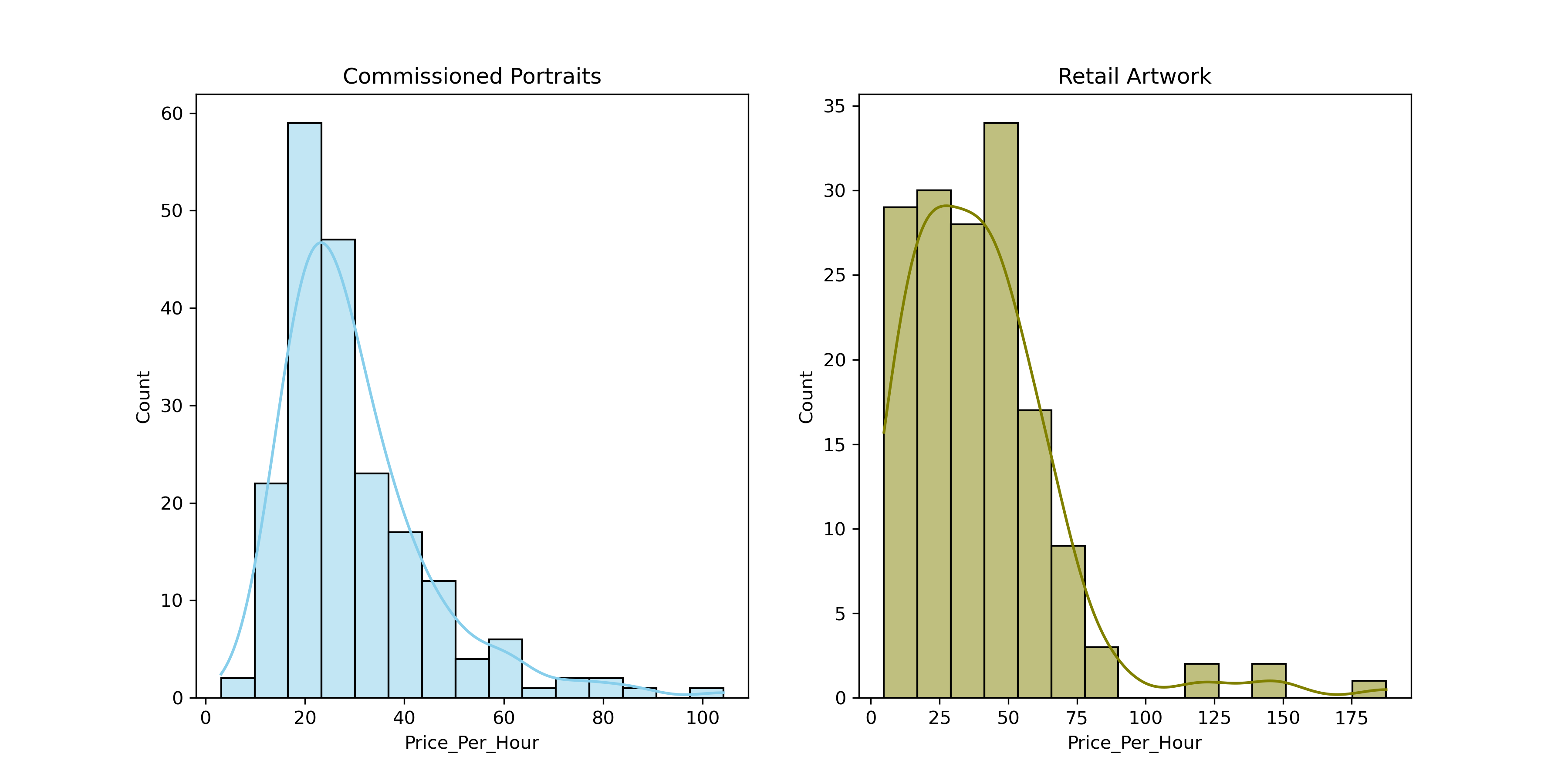
This indicates that pricing for commissioned portraits is reasonably well clustered with a mean of around 25 USD/hour for commissioned portraits and a more spread-out distribution with a mean of around 35 USD/hour for retail artwork. But why are the prices for retail artwork so spread out?
Is Pricing Consistent with the Painting Size?
Let's look at the price per area instead:
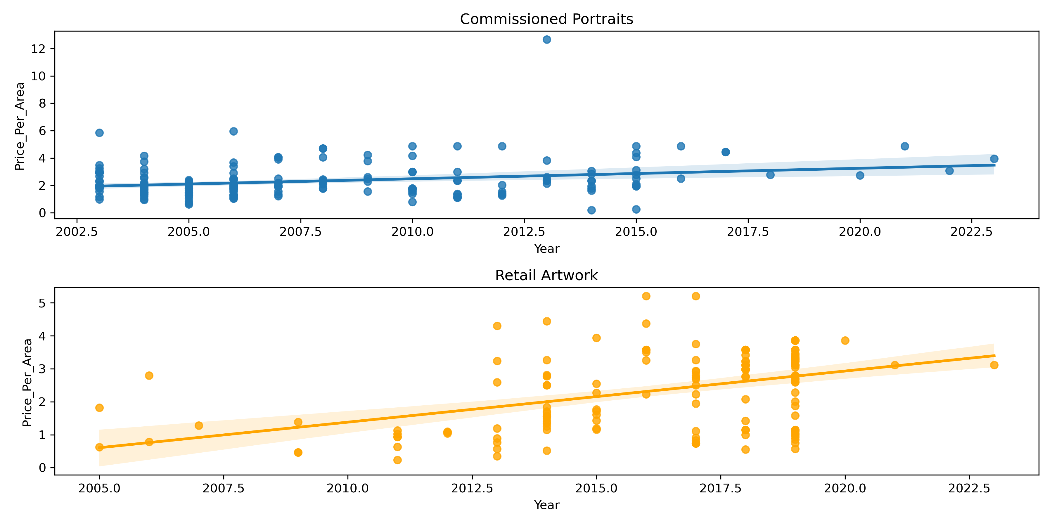
The regression lines seem to indicate that commissioned paintings and retail artwork are currently equivalent in terms of price per unit canvas size, but that the price of retail artwork is increasing at a faster rate than commissioned portraits.
The retail artwork data also looks more spread out in this plot, so let's try to understand why.
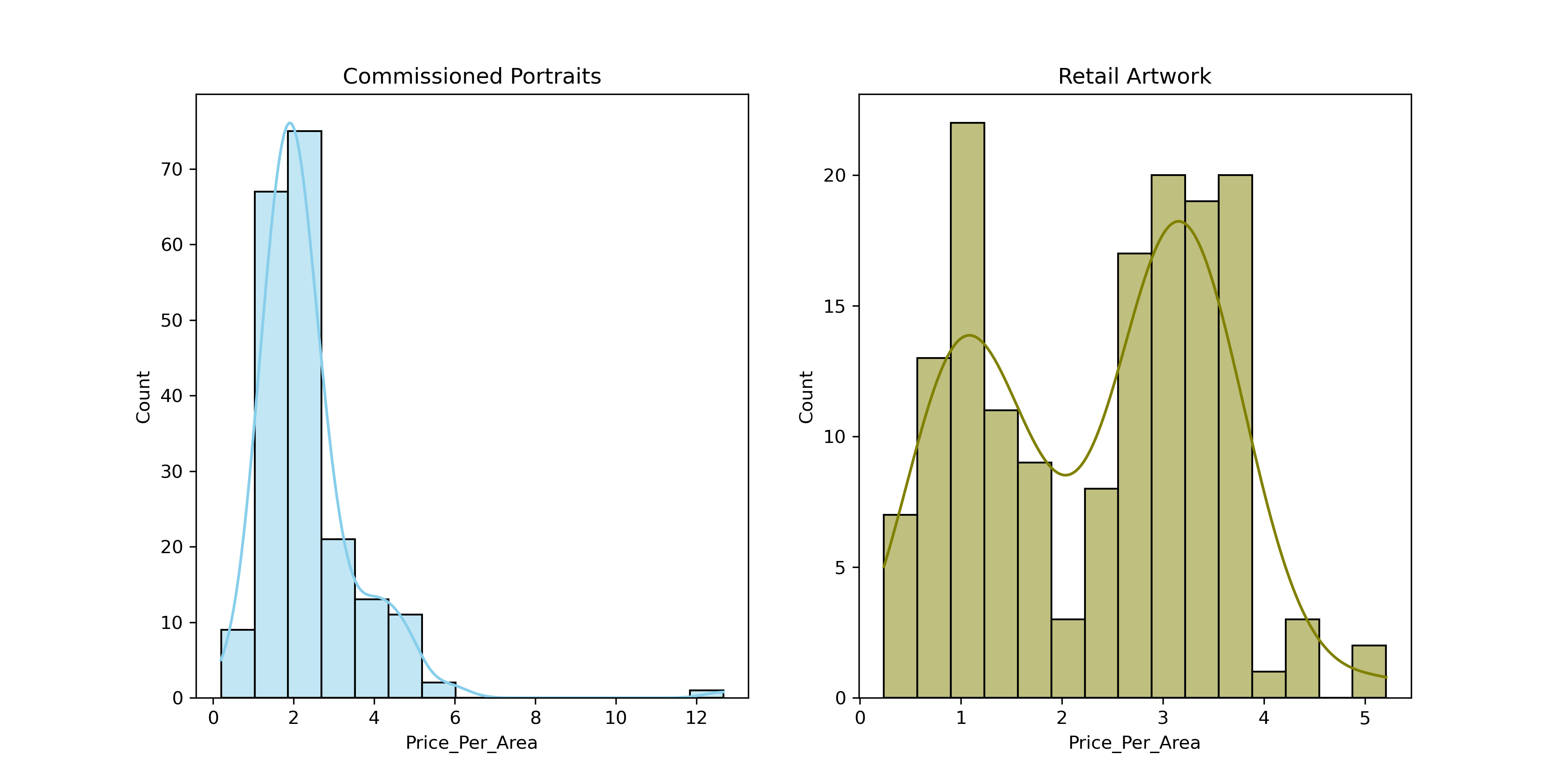
The distribution of price per area for commissioned portraits is evidently well grouped. For retail artwork, there are two distinct groupings—it takes the form of camel humps in the KDE curve. This can be explained by selling both framed and unframed paintings (I've provided details of this in the detailed analysis which you can find on my GitHub page).
Commissioned paintings are always sold unframed. For framed retail artwork, the price by unit canvas size is ~50% greater than that for commissioned paintings although I have to cover the cost of the frame, so there's probably less separation than this.
Can We Predict Time to Complete?
I'm interested in being able to estimate how long a portrait will take to complete. I could use that to help price it correctly and to figure out my studio workload with more accuracy.
Along with price and size, I have tracked the amount of time it takes to finish each portrait, although the data is less precise.
Before we start regression, let's quickly plot the relationship between Actual Time and Year to confirm my suspicion that there's no direct relationship between the two. Portraits of people are the most time-consuming and difficult to complete, so we'll focus on those for now.
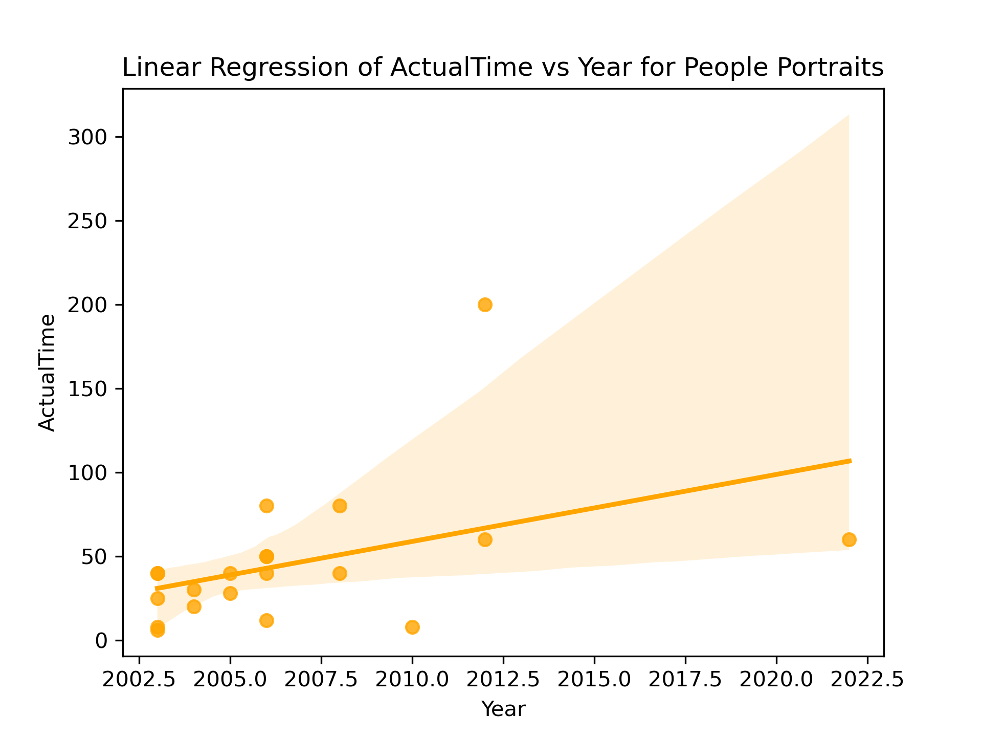
This plot indicates there might be a direct correlation between Actual Time and Year, but I want to inspect the data more carefully: I know that the time spent increases with number of subjects and with area, so let's find a way to show the trends in those over time by looking at:
- Actual Time per Unit Area vs. Year
- Actual Time per Head vs. Year
Before we start a more complex regression, let's plot the relationships between the variables.
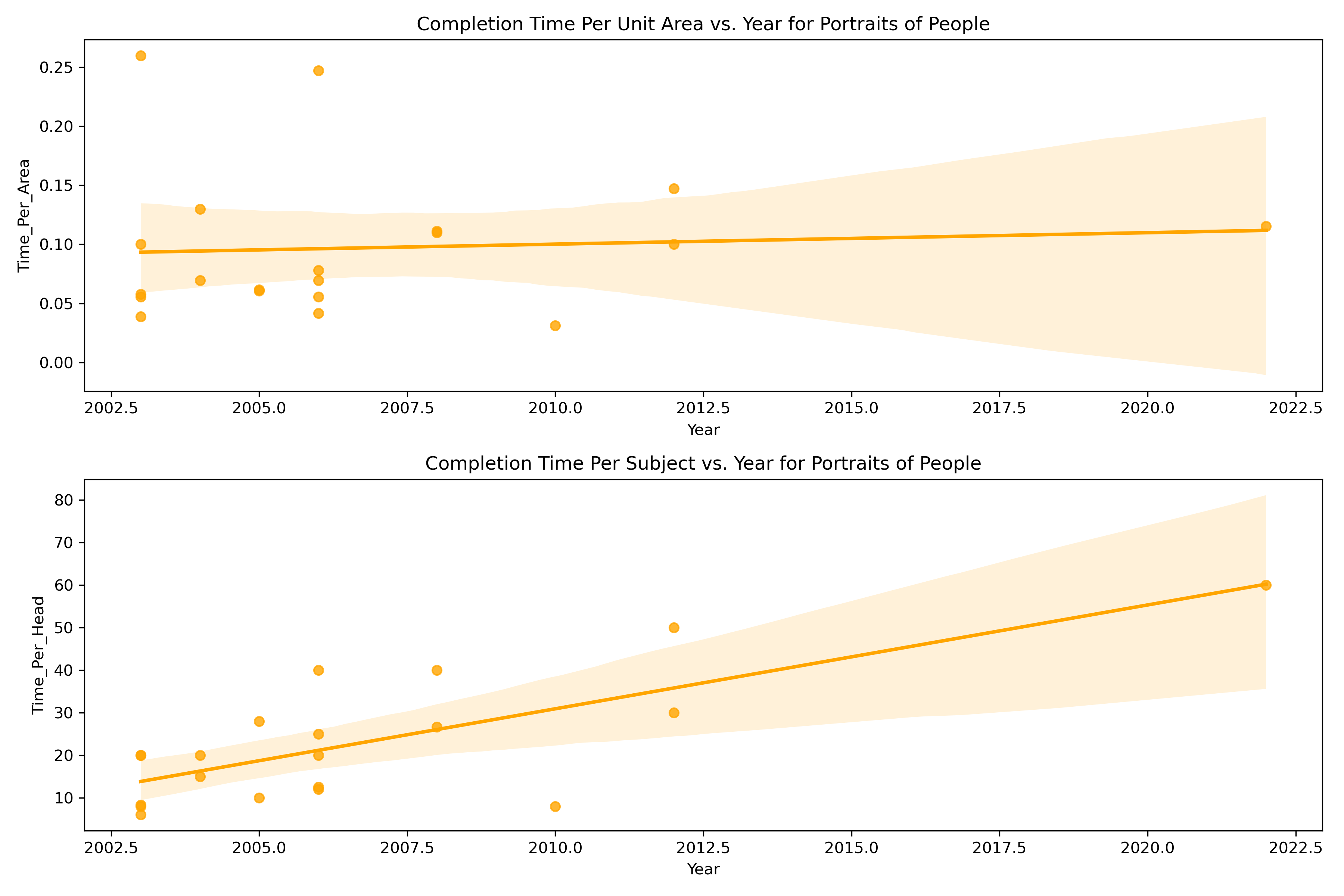
There are several outliers in the data, which might be due to misclassification, but there's also an aspect of the portrait creation process at work here: some painting projects simply take longer than others and it can be difficult to predict which ones those will be in advance.
A multi-variable linear regression yields the following:
The R2 value is:  0.6059059359108192
The intercept is: -5714.259688343059
The coefficient for Year is 2.846720892057734
The coefficient for Area is 0.05614672115382439
The coefficient for NumSubjects is 9.431313897337578
Which is a reasonably good fit. Let's check the model by estimating how long it would take to complete a portrait of one person on a 20x26 canvas in 2025.
# Put data into variables
year = 2025
area = 20 * 26
num_subjects = 1

# Predict price
time = intercept + coefficients[0] * year + coefficients[1] * area + coefficients[2] * num_subjects

print('The predicted time is: ', time.round(1), 'hours')
The predicted time is:  89.0 hours
That seems like a very good estimate. Now, let's work on prices.
Can We Predict the Price of a Dog Portrait?
One thing that will have been obvious in the previous plots is that the data I have for people portraits is rather sparse. I have much more data relating to dog portraits than those of other subjects, so it's natural choice to make them the target for this next analysis.
I tend to price portraits based on a combination of my historical data and a rough assessment of how difficult I assess they will be to complete. In the absence of a 'difficulty' rating, we'll examine the correlation between year, area, number of subjects and price. This requires another multi-valued linear regression.
First, we'll do a check to confirm my suspicion that Price vs. Year doesn't provide a meaningful regression line.
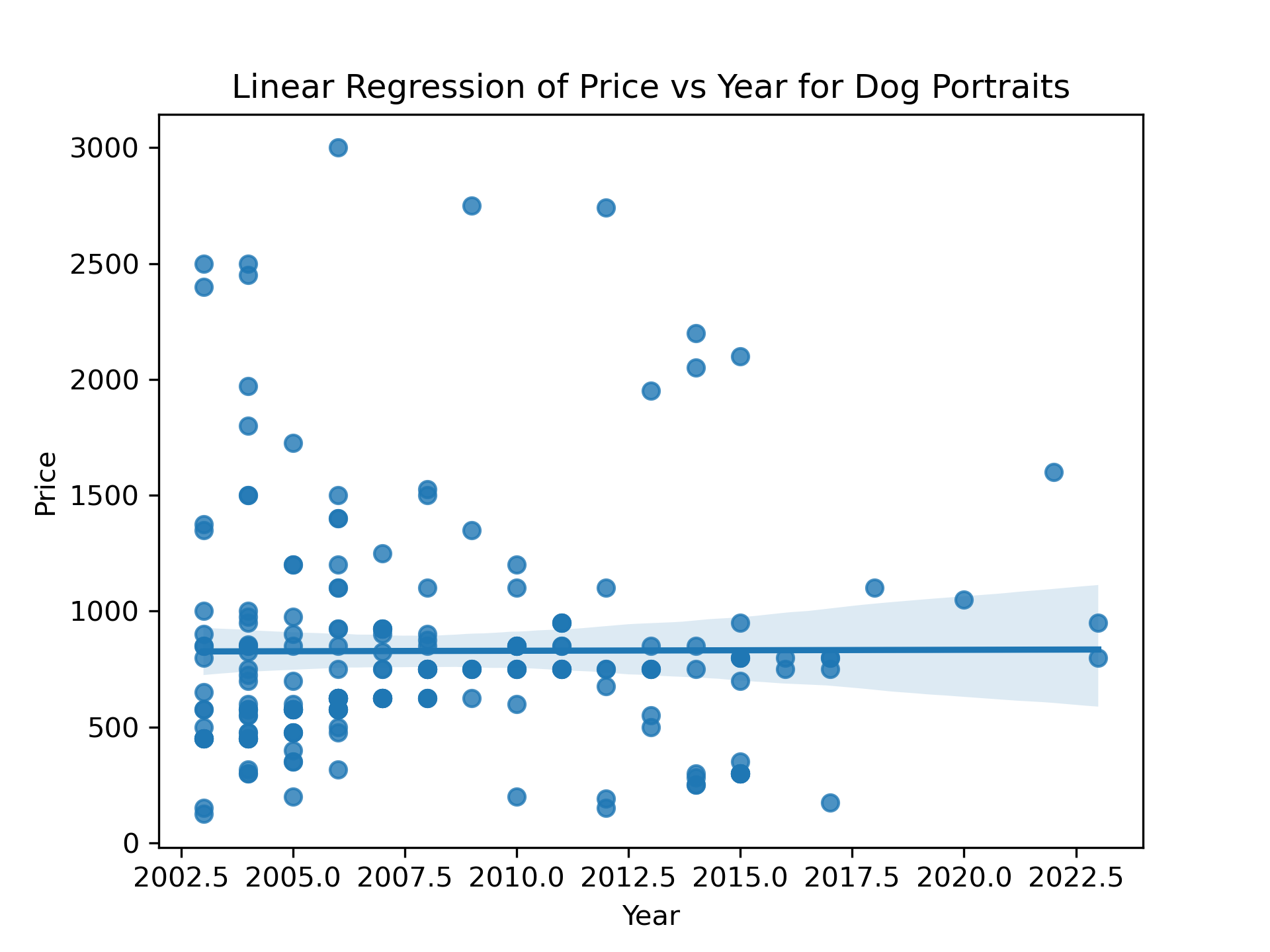
That's a relationship that's not going to provide us with any meaningful insights.
However, I do have an idea what to focus on. Prices tend to be higher for larger canvas sizes (for example, I might be painting a whole body rather than just a head and shoulders portrait), and prices tend to be higher for multi-subject portraits (it takes more effort to paint two dogs than it does to paint one). In addition, prices are likely to increase over time. We can therefore plot:
- Price per Area vs Year
- Price per Head vs Year
One further thing:
In 2010 or so, I started doing two grades of portrait—a sketch portrait that started at 400 USD per head and a formal portrait that started at 700-800 USD. The data didn't make much sense with the sketch portraits included, so I removed them.
Before this, I didn't officially do sketch vs. formal portraits, but there were a few lower cost portraits in the mix. I removed these, too.
Before we start a more complex regression, let's plot the relationships between the variables.
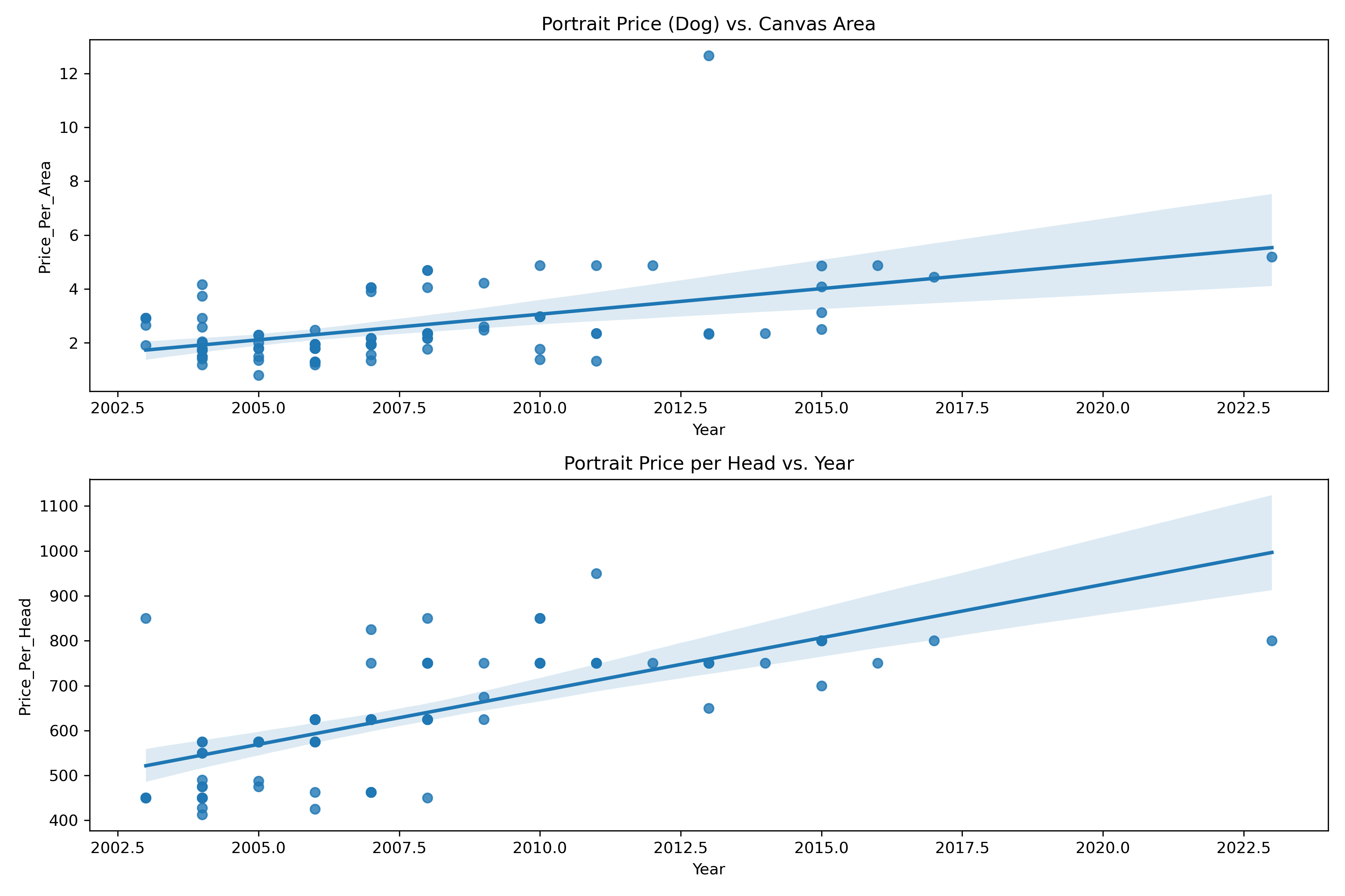
Based on these plots, we can relate price, area, number of subjects and year. Now we can try a multi-variable linear regression—that should give use enough information to make price predictions.
The R2 value is:  0.8678301344450077
The intercept is: -52433.1759966182
The coefficient for Year is 26.194149928731722
The coefficient for Area is 0.12031041246223617
The coefficient for NumSubjects is 452.2857750676249
That produces a strong correlation. Let's estimate the cost of a two-dog portrait on a 20x24 canvas in 2025 using the coefficients that were calculated above:
# Put data into variables
year = 2025
area = 20 * 24
num_subjects = 2

# Predict price
price = intercept + coefficients[0] * year + coefficients[1] * area + coefficients[2] * num_subjects

print('The predicted price is : $', price.round(2))
The predicted price is : $ 1572.3
Which is in the right ballpark, although a little lower than I would like it to be.
Can we Predict the Price of a Portrait Using Polynomial Regression?
While straight line fitting looks good, I also want to examine polynomial curve fitting.
It has an extra degree of difficulty over straight-line fitting: we don't know what order of polynomial to use.
The way around this is to try different degrees of polynomial in turn to see which works best. But here lies a problem—as the degree of the polynomial increases, the regression can become over-fit (it tries to take all the noise into account). The solution is to split the data into a test group and a training group. The training data is used to come up with a regression curve, then test data is used to validate the model.
Here is the result of doing that for the dog portrait commissions:
| Degree | Training RMSE | Test RMSE |
|---|---|---|
| 1 | 111.54 | 122.51 |
| 2 | 89.91 | 116.20 |
| 3 | 67.65 | 137.10 |
The results show that the polynomial rapidly becomes overfit at third order and higher. We can visualize that by plotting the training RMSE against the test RMSE.
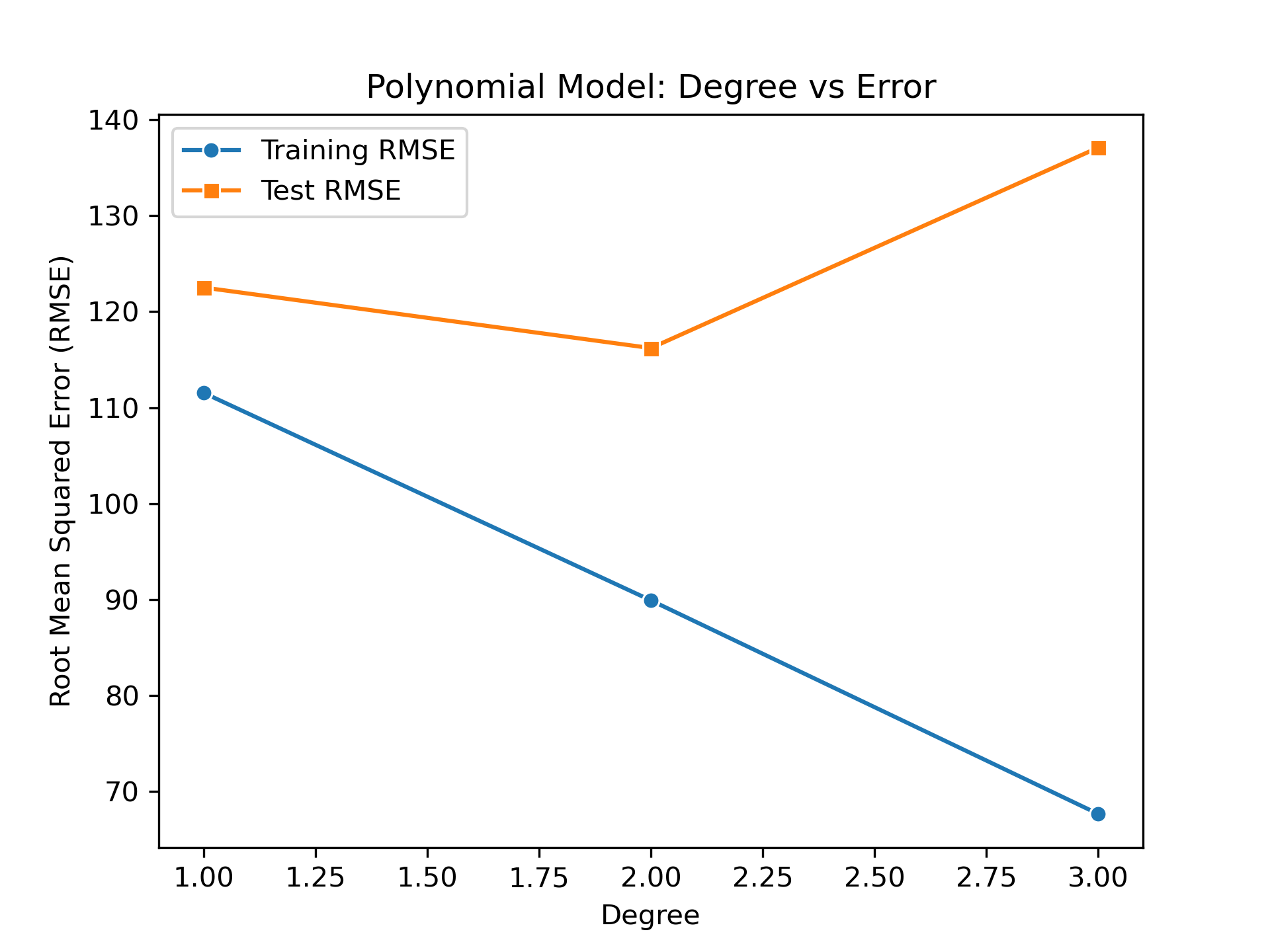
The optimum polynomial appears to be second order. Clearly, the sparse portrait data after 2019 (thanks, COVID!), makes fitting in this time period and projections into the future a challenge.
Predicting a Price Using a Second Order Polynomial
Let's fit a second order polynomial to the entire data set.
Intercept: -5312758.340217695
Coefficients:
1: 0.0
Year: 5288.709863302076
Area: -60.30536117705008
NumSubjects: -39419.184523918404
Year^2: -1.3161292986936226
Year Area: 0.030290810859441963
Year NumSubjects: 19.753826213429235
Area^2: -0.0001778904048839471
Area NumSubjects: -0.10540792452618564
NumSubjects^2: 73.93718308278852
R² score: 0.9086869357574229
That produces a stronger correlation than the multi-variable linear regression. An interesting result is that the model predicts a price decline in the future (the coefficient for Year^2 is negative) — this comes from a mild overfitting of the training data combined with the lack of data after 2019.
Still, it might get us a price estimate in the right ballpark. As before, let's estimate the cost of a two-dog portrait on a 20x24 canvas in 2025 using the coefficients that were calculated above. Unfortunately, it's much more complex than the linear calculation:
# Put data into variables
year = 2025
area = 20 * 24
num_subjects = 2

# Predict price
price = intercept + (coefficients[1] * year) + (coefficients[2] * area) + (coefficients[3] * num_subjects) + \
        (coefficients[4] * year * year) + (coefficients[5] * year * area) + (coefficients[6] * year * num_subjects) + \
        (coefficients[7] * area * area) + (coefficients[8] * area * num_subjects) + (coefficients[9] * num_subjects * num_subjects)

print('The predicted price is : $', price.round(2))
The predicted price is : $ 1740.72
That's a very good estimate—right around where I would try to price a 20x24 two dog portrait of moderate complexity.
Footnotes
Privacy
Wherever possible, the data has been anonymized.
Where is the Data From?
As soon as I started doing art full time, I built an application to help me manage my customer base, do invoicing and track expenses. With a few tweaks, that system has been in continual use for 20 years. The data was extracted from there via SQL queries and saved to an Excel spreadsheet, where I did some simple cleanup before loading it into Pandas.
How Did I Clean and Analyze the Data?
You can see the full analysis I did on my GitHub page: prices and timing, time predictions and price predictions. I'd encourage you to take a glance if you're interested in how this is done.
To start, some data cleanup was required. There were a few records that had null values in otherwise important fields, an outlier in the price field (a very large painting that would otherwise skew the analysis) and some of the fields needed to be converted to numeric data.
The data analysis was done with Python, Pandas, and the Scikit-Learn machine learning library. Plotting was done with Matplotlib and the Seaborn libraries.
A briefer version of this article was also published on LinkedIn
Simon Bland: 09 Feb 2025